Saturday, December 17, 2011

Matching image colors with Texturewerke

In the last post I demonstrated how to use TextureWerke for masked polynome high-pass filtering. In addition to that, TextureWerke 0.1 has another feature - matching colors between two (masked) images.

Workflow

Let's start with two images of stone wall we want to merge into one texture:

First image - a plain wall

Second image - a corner made of bricks

As you can see (among other things) the images have a bit different colors - the first one has more contrast and red. The bright background of the second picture influenced camera color adjustment logic so that the wall is more gray and has less contrast.
We will correct this automatically. First we move both photos to the same image (not necessary, but easier to compare) and add masks. We mask out all details that we do not want to influence final color - i.e. roof, shaded areas, brick structures, grass and background.

Masked images on top to each other.

Next we select the masked layer whose colors we want to change (Layer 2), invoke TextureWerke and choose color matching mode.

TextureWerke dialog window in color mode

Template is the (masked) layer whose color profile we want to emulate in selected layer.
Blurring reduces the noisiness of distribution curves and thus helps to overcome artefacts resulting from different sharpness of images. On the other hand it may mask out certain differences in color distribution and thus reduce the matching quality. You can always try and use what gives the best results.
And at last we apply the filter.

Image with adjusted colors

As you can see, the overall color and contrast of the (stone part of) wall matches with template image. On the other hand the areas that were masked out (bricks, backround...) are now completely off. But probably we did not want to use these anyways - except bricks maybe - but these can easily be copied and pasted from the original, and adjusted separately.

FYI: Internally the algorithm works by comparing pairwise the cumulative distributions of each image channel (R,G,B,A) and building a transfer function that translates the values with one distribution to the values with another (template) distribution.

And that's all. Have fun!

Thursday, December 8, 2011

Texturewerke 0.1

While doing textures for Shinya (the game with Khayyam/Sehle engine) I got frustrated with GIMP built-in tools and plug-ins available for texturing and decided to write my own tool Texturewerke. The initial version is now available for download from SourceForge:
At moment it can do two things:
  1. Adjust the colors of one (masked) image so it matches as well as possible with another. Thus you do not have to manually adjust color curves to merge several photographs into the same texture.
  2. Filter out low frequencies from image (while keeping the average intact). This can be used both for the creation of seamless textures and for removing shade gradient from uniform surfaces (like walls, doors, whiteboards...) Highpass filter supports masking (in polynome mode), so you can mask out those details whose contribution you want to ignore (like pictures on wall).
Below is one possible usage scenario of Texturewerke highpass filter.

Polynomic highpass filter with masking

We want to use the following image as a texture. Unfortunately the background color is non-uniform and adjusting it by hand is boring work

The original image - notice the non-uniform shading of the wall
We select the are that we want to have uniform color (the wall). It does not have to be precise - the filter samples few thousand points from target area and thus small regions of wrong color do not disturb the result much.
In given case I used magic want to select white and then added and subtracted few rectangles.

Target region selected
Now we turn target region into mask, bu choosing "Add Layer Mask" from Layer menu.

Target region turned into mask
Next we invoke Texturewerke plugin and select "Lowpass" filter and "Polynome" mode.

The Texturewerke dialog window
It blurs image (internally) before calculating polynome approximation. The optimal size of kernel depends on image and the number of samples used. As general rule - the more samples it uses, the smaller can be the kernel.
Next we apply filter.

Masked image after applying polynome filter
As you can see, the unmasked area has almost uniform color/bightness now.
As the last thing, we delete (or turn off layer mask).


The final image - wall color is now uniform
 And the final image has now nice uniform wall color.

There are few things to notice:
  • Polynome mode tries to approximate the average color of the image by two-dimensional polynome (up to 4th degree). The approximation process guarantees the correct behavior of the polynome only inside target region - the higher is its degree the faster it goes "wild" outside. Thus if you mask out some edges of the image the results probably will not look nice for anything above quadratic (2th order).
  • The unmasked area has to be at least 10% of original image
  • Samples are drawn randomly from unmasked area.
  • There is another highpass filter mode "blur", that subtracts blurred (lowpass) version of the same image. It does not support masking - but it may be more useful for the generation of highly uniform images (like grass and sand textures).

Have fun!

Tuesday, October 4, 2011

Reflective water with GLSL, Part II

In the first part I explained how to implement a basic reflective surface. But as we could see, it was very poor approximation of true water, looking more like mirror lying on the ground.  First because real water is almost never completely still. But it is also not perfect mirror - depending on viewing angle we can see more or less into the water.
Before going to implementing ripples I'll show how to adjust water shaders so the angle-dependency of reflection strength is taken into account. And being already there, how to fake the light attenuation/scattering in water so it is not crystal-clear but has more realistic color.

1. The relation of reflectivity and viewing angle

If you imagine looking at water body from different angles it should be obvious, that the lower is viewing angle the more light it reflects. Sea may look almost like perfect mirror during tranquil sunset - but if you are looking daytime from the top of a cliff, you can see the blueish-greenish color of water and only a little reflection.

The reflectivity of water comes from the difference in refractive indexes of air and water. As the speed of light is different in these mediums, some light is reflected and the light entering water changes slightly its direction - the latter is called refraction. Refraction is another phenomenon that can add realism, but we will not try to simulate it here.

A schematic diagram of reflection and refraction

Mathematically the amount of light reflected from the surface of water is described by Fresnel equations:

Fresnel reflection equations (source Wikipedia)

Rs and Rt are the reflectance values of vertically and horizontally polarized light.
θi and θt are the angles between the surface normal and incident and refracted rays.
n1 and n2 are the refractive indices of two media - in our case air and water. The relevant values are:

n1 = 1.000277 ≈ 1
n2 = 1.3330

We do not need θt because it can be derived from θi and refractive indices using Snell's law - look at the rightmost part of equations.
The reflectance values are different for differently polarized light. This explains the magic behind anti-glare sunglasses and optical filters - they cut off vertically polarized light, that is much more strongly reflected.
It is also interesting to know that skylight is in fact somewhat polarized. But for our simulation we ignore this and treat all light as the uniform mix of both polarizations. In that case, the total reflectance can be simply calculated as:

R = (Rs + Rt) / 2

The full Fresnel equation above is a bit too complex for our shaders. It is physically correct - but our goal is natural or good-looking scene and we are ready to sacrify a little here ad there to save shader instructions for other things.
There is quite simple approximation available. Take a look at the following graph:

Fresnel reflectance values Rs, Rp and R (blue, red, yellow) and our approximation (green) 
The green line represents function:

R = Rmin + (1 - Rmin) * (1- cos θi)5

That can be used as good approximation.
Rmin is 0.02 for real water, but you may want to increase it to something like 0.1 or even more, unless you have very good HDR implementation. The problem is that real sky is really bright - if you are using dimmed down version of sky, its reflection is not visible at all from high angles.

That's it. Now we have reflectance value calculated - but we cannot yet update our shaders. Unlike in our previous lesson, where the reflection was all that had to be rendered, we now have to render the water itself too - unless the reflectance is exactly 1.

2. Rendering water

Water is normally dense medium and strongly scatters light. The actual formula is quite complex and depends on the amount of different chemical compounds (such as oxygen, humic acids) and various inorganic (such as clay) and organic (like plankton) particles in water. But our goal is not to simulate procedurally the color and turbidity of water, but instead find a meaningful set of descriptive parameters, that will give us good enough approximation.

Scattering changes the intensity of light (ray) in two ways:
  • Out-scattering - if ray of light goes through medium, some fraction of light is scattered away from direct path and thus the final amount of light is lower.
  • In-scattering - as light is scattered to all directions, some light from rays originally going other directions is scattered to the direction of the ray of interest.
Because of out-scattering the bottom of deep water body is dark. Because of in-scattering objects inside water seem "tinted" with water color.

Scattering in water. A - in-scattering. B - out-scattering.
In addition to scattering there is one more phenomenon causing less light to come from water - it is internal reflection. As light hits the bottom of water body or objects inside it and goes upwards from there, some of it is mirrored back into water from the air-water phase surface.
We ignore this at moment and will use shortcut - instead of adding together the light coming from inside water and light from reflection, we draw the latter as semitransparent surface using reflectance as alpha value. Thus the higher is reflectance, the lower is the effect of light from inside water - which is generally correct, because the internal and external reflectance values are correlated.

How good our water formula can be depends on whether we can read the color and depth values of the bottom of water body or underwater objects in shader or not. Here I present a simple approach, that does not use them, but instead adds the color of water to the reflection image.

We ignore the exact scattering equations, that involve multiple integrals and instead combine the "tint" of water with the color of reflection (that is semitransparent now) and then render them as semitransparent surface over the already rendered bottom of water. For this I use a very simple formula:

Ctint = Cwater * (Omin + (1 - Omin) * sqrt (min (thickness / Dopaque, 1)))

Ctint is the color that water adds to objects (premultiplied)
Cwater is the color of opaque water column
Omin is the minimal opacity of water. It should be 0 for realistic simulation, but in reality values 0.1-0.2 give overall better effect.
Dopaque is the depth of water column, that becomes fully opaque. The reasonable value is 2 m for freshwater bodies - the smaller the better, as it helps to hide the lack of refraction.
thickness is the thickness of water in given direction until bottom or some underwater object is hit.

Calculating thickness is tricky. The technically correct way would be to trace ray in refracted direction until bottom (line AC in following figure) - but we cannot afford to do that.
If you can use depth buffer, you can ignore refraction and calculate the distance the original ray would cover underwater (line AD). This overestimates the thickness, but as the effect only becomes noticeable at low viewing angle, where reflection dominates, it should look quite good.
Here I will use even simpler approximation. Just find the depth of water under given point of surface (point B on following figure), and pretend that water has uniform depth (line AB1). It underestimates depth at the slopes directed away from viewer and overestimates at slopes directed to viewer, but if the bottom of water is reasonably smooth it is not too bad.

A diagram of different possible methods for water thickness calculation
How to get the actual water depth under given point?
Recall the previous tutorial. We set the Z coordinate of vertex to 0 (i.e. flatten our object), but kept the full original vertex coordinate in interpolatedVertexDepth.
Thus if the object being rendered as water is actually the bottom of water body, it will render as flat surface, but we have access to the original Z coordinate of it. In other words - the water depth.
Another approach would be to encode water depth into another vertex attribute. It has some good points - like no need to separate the bottom of water body from other terrain and the possibility to hand-code depth.

Once we have calculated water thickness with whatever method applicable, we treat the tint color as another semitransparent layer, lying directly beneath the reflection layer. The final color and alpha values can be calculated by standard alpha blending formula:

C = Areflection * Creflection + (1 - Areflection) * Cwater
A = Areflection + (1 - Areflection) * Awater

Where C and A are color and alpha values.
If the resulting alpha is below 1, bottom or underwater objects are partially visible.

3. Shaders

There is no need to change vertex shader.

Fragment shader:

uniform mat4 o2v_projection_reflection;
uniform sampler2D reflection_sampler;
uniform vec3 eye_object;
uniform float min_opacity, opaque_depth, opaque_color;

varying vec3 interpolatedVertexObject;

void main()
{
    // Vertex on water surface
    vec3 surfaceVertex = vec3(interpolatedVertexObject.xy, 0.0);
    // Reflection angle
    vec3 vertex2Eye = normalize (eye_object - surfaceVertex );
    float cosT1 = vertex2Eye.z;
    // Reflectance
    float c = 1.0 - cosT1;
    float R = min_reflectivity + (1.0 - min_reflectivity) * c * c * c * c * c;

    // Water density
    float depth = -interpolatedVertexObject.z;
    float thickness = depth / max (cosT1, 0.01);
    float dWater = min_opacity + (1.0 - min_opacity) * sqrt (min (thickness / opaque_depth, 1.0));
    // Premultiply
    vec3 waterColor = opaque_color * dWater;

    vec4 vClipReflection = o2v_projection_reflection * vec4(interpolatedVertexObject , 1.0);
    vec2 vDeviceReflection = vClipReflection.st / vClipReflection.q;
    vec2 vTextureReflection = vec2(0.5, 0.5) + 0.5 * vDeviceReflection;

    vec4 reflectionTextureColor = texture2D (reflection_sampler, vTextureReflection);
    // Framebuffer reflection can have alpha > 1
    reflectionTextureColor.a = 1.0;

    // Combine colors
    vec3 color = (1.0 - R) * waterColor + R * reflectionTextureColor.rgb;
    float alpha = R + (1.0 - R) * dWater;

    gl_FragColor = vec4(color, alpha);}

We have added another uniform (in addition to water color and opacity ones) - eye_object, that is simply camera position relative to water object local coordinate system.

And real-time image from Shinya:

Simple scene from Shinya with partial reflection and water opacity 

Now it is a bit better than last time - but still artificial and lifeless. Next time I show, how to make it live - i.e. add waves or ripples.

Part 1 - reflective surface

Have fun!


Friday, September 16, 2011

Reflective water with GLSL, Part I

Being it for physical accuracy or setting mood in game, water and reflections are something that can add lot to your rendering engine. While true reflections can only be done with ray-tracing, one can achieve surprisingly nice approximations by using quite simple scene setup and some GPU programming.

Good water simulation should have at least the following features:
  • True reflection (with correct parallax)
  • Clipping of underwater objects on reflection image
  • View angle dependent transparency/reflectivity of water
  • Ripples and/or waves
  • Water scattering (i.e. water becoming gradually opaque as depth increases)
 Some more things, that can make things nicer but are not as visible, are:
  • Refraction
  • Caustics - i.e. light spots at the bottom of shallow water
  • Reflected light - i.e. light spots reflected to objects near water
At moment I have only implemented features from the first list into Khayyam/Sehle/Shinya code. You can look at my previous post for some in-engine images.
Here I will describe the mathematics behind the scenes and give step-by-step guide to writing your own water system/object/rendering pass.

1.Rendering reflection texture

Water without reflection looks totally uninteresting - just like any other semitransparent surface. Thus we start from implementing reflection and later go on to other effects.

1.1. Parallax
Even if you have until now managed to render you scene in single pass, from this point on you need at least two passes (actually at least N+1, where N is the number of visible reflective surfaces).

The reason is, that unfortunately we cannot recycle our main scene image for reflections. First because it could make view frustum insanely large (for example - if viewing the water surface from high angle we see only ground and water in our main view, but mostly sky in reflection). And second because of parallax. The reflection is unfortunately not the perfect copy of reflected scene, but copy of the view of the same scene from different viewpoint. The following image illustrates this.

A diagram explaining the parallax effect on reflected image

It means that you need to have rendering to texture set up and working. We will render reflection to texture and later use this texture while rendering the water surface in main scene.

Thus, to get reflection texture we first have to render our scene from the reflected camera viewpoint  P' to texture. First we have to find the reflected camera position - or more precisely the reflected view matrix (because we need camera orientation too in addition to the position).
This can be done with the following formula:

M'camera = Mreflection * Mcamera

Where Mreflection is the reflection matrix of mirror surface. It can trivially be calculated from the position of reflection plane:

              | 1-2Nx2   -2NxNy  -2NxNz  -2NxD |
Mreflection = |  -2NxNy 1-2Ny2   -2NyNz  -2NyD |
              |  -2NxNz  -2NyNz 1-2Nz2   -2NzD |
              |    0       0       0       1   |

Where (Nx,Ny,Nz,D) are the coefficients of plane equation (xNx + yNy + zNz + D = 0). Notice, that (Nx,Ny,Nz) is also the normal vector of given plane.

Mcamera is the transformation of camera as if it would be "normal" object in scene. To get ModelView matrix you will need the inverse of it.

1.2. Mirrored geometry
Actually we cheated a little in the previous image. We rotated the mirrored image 180º to make it more similar to the original image, so the effect of parallax can be seen. The actual mirrored image looks like this:
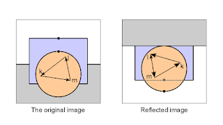
Different winding order on mirrored image
Notice, that the winding order of polygons in image is flipped on mirrored image - i.e. the triangle is oriented CCW on original but CW on reflection.

This may or may not be problem for you. If all your materials are double sided (i.e. you do not do back face culling) or if you can set up rendering pipeline in such a way, that you can change culling direction it is OK. In my case though, I prefer to keep culling always on and have forward-facing always defined as CCW. So something has to be done with the reflected image - or otherwise geometry will not render properly.

We will exploit the feature that camera is always (at least in most applications) rectangular and centered around view direction. Thus we can just flip camera in Y direction and the winding order will be correct again (it flips reflected image so it looks like (3) on the first picture).
This can be done with one more reflection matrix:

M''camera = Mreflection * Mcamera * Mflip

Where Mflip is simply another reflection matrix that does reflection over XZ plane.
Now if we render mirrored image using M''camera as camera matrix, pipeline can be left intact. We, of course, have to save this matrix for later reference, because it is needed to properly map our texture to water object in main render stage.

1.3. Underwater clipping
Take a look at the following picture:
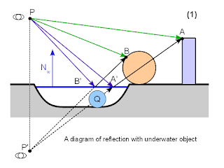
A reflection with underwater object


We have added an underwater object Q to our scene. Now it should not appear on reflection, because it does not block the actual reflection rays PB'B and PA'A. But we are not doing ray-tracing. We are instead moving camera to mirrored viewpoint P' and rendering reflection like normal image. But as you can see, the object Q blocks ray P'A'A and thus would show up in our reflection.

Thus we have to make sure, that nothing that is under the reflection plane (water surface) will show up in mirror rendering. This can be achieved in three different ways:
  1. Use additional clipping plane on GPU. It can be very fast or very slow - depending on card and driver used.
  2. Use oblique projection matrix during reflection rendering. You can read more about it here. This is cool technique, but personally I have never got it to work well enough because it messes up camera far plane.
  3. Clip manually in pixel shaders. It wastes some GPU cycles, but is otherwise easy and foolproof.
I went with option (3) because oblique projection matrix did not seem to play well with wide camera angles (far plane moved through infinity creating all kinds of weird effects). The clipping itself is as easy as adding the following code at the beginning of all pixel shaders (or more precisely the ones that are used for reflectable objects):

uniform vec4 clip_plane;
varying vec3 interpolatedVertexEye;

void main()
{ 
    float clipPos = dot (interpolatedVertexEye, clip_plane.xyz) + clip_plane.w;
    if (clipPos < 0.0) {
        discard;
    }
...
}

Of course you have to supply your shader with clip_plane and calculate interpolatedVertexEye in vertex shader (it is simply vertex coordinate in view/eye space: VertexEye = Mmodelview * Vertex). If you do not need clipping, simply set clip_plane normal (xyz) to zero and all pixels will be rendered.

1.4. Putting it all together
Before starting the main render pass (being it forward or deferred) do the following:
  1. Create list of all objects that need reflections (and the parameters of all reflection planes). Then for each reflection plane:
  2. Calculate the reflected camera matrix
    M''camera = Mreflection * Mcamera
    * Mflip
  3. Set up camera matrices (you can optimize rendering by using clipped projection matrix, but this will not be discussed here).
  4. Set clipping plane to reflection plane
  5. Render full scene
  6. Save the rendered image as texture to be used with reflective object
If you are using HDR you should not tone-map reflection texture - unless you want to achieve some very specific effect.
2. Rendering reflective object

This is actually quite easy - provided that you have at hand all necessary parameters. You have still to decide at which render stage to do this. I use transparent stage, as water is basically just one semi-transparent surface in scene, but you can add another pass before or after transparency as well.

You will need at hand:
  • Reflected camera matrix M''camera
  • Projection matrix you used to render reflection Mprojectionreflection (normally this is the same projection that you use for main camera)
  • Reflection texture

2.1. Vertex shader

attribute vec3 vertex;

uniform mat4 o2v_projection;

varying vec3 interpolatedVertexObject;

void main()
{
	gl_Position = o2v_projection * vec4(vertex.xy, 0.0, 1.0);
	interpolatedVertexObject = vertex;
}

We add another constraint here - water surface will be at XY plane of the object local coordinate system. It is strictly not necessary if you have the proper reflection plane, but I found it easier that way. Just use XY plane as reflection plane and place your object (water body) appropriately.

Actually this allows us to do another cool trick. We can use the bottom of water body (i.e. river, lake..) as our water object. It will be flattened in shader, but we can use the Z data to determine the depth of water at given point. But more about this in next part. 

o2v_projection is simply my name for composite matrix Projection * ModelView. I prefer to name matrices with mnemonic names, describing the coordinate system transformations they do - in given case it is Object To View, multiplied with Projection. 

interpolatedVertexObject is simply vertex coordinate in object local coordinate system - we will need it to do lookup onto reflection texture.

2.2. Fragment shader

uniform mat4 o2v_projection_reflection;
uniform sampler2D reflection_sampler;

varying vec3 interpolatedVertexObject;

void main()
{
	vec4 vClipReflection = o2v_projection_reflection * vec4(interpolatedVertexObject.xy, 0.0 , 1.0);
	vec2 vDeviceReflection = vClipReflection.st / vClipReflection.q;
	vec2 vTextureReflection = vec2(0.5, 0.5) + 0.5 * vDeviceReflection;

	vec4 reflectionTextureColor = texture2D (reflection_sampler, vTextureReflection);

	// Framebuffer reflection can have alpha > 1
	reflectionTextureColor.a = 1.0;

	gl_FragColor = reflectionTextureColor;
}

o2v_projection_reflection is the composite matrix Projection * ModelView as it was used during reflection rendering. I.e:

Mprojectionreflection * (M''camera)-1 * Mobject

Like the name implies, it transforms from the object coordinate system to the clip coordinate system of reflection camera.

In fragment shader we simply repeat the full transform pipeline during reflection rendering and use final 2D coordinates for texture lookup. For this we need initial, untransformed object vertices - thus they are interpolated from vertex shader (interpolatedVertexObject).

I'll set reflection alpha to 1.0 because I use HDR buffers and due to additive blending the final alpha can have some very weird values there.

And the rendered image:

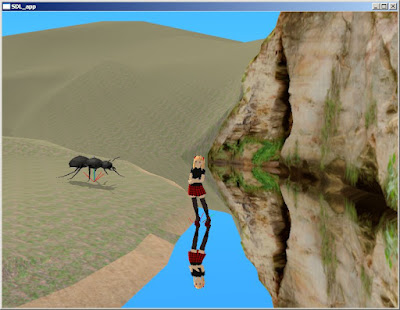
Simple scene from Shinya showing water as perfect mirror

Not very realistic?
Up to now we have implemented water as perfect mirror. This is very far from reality (look at the feature list in the first section).

In the next parts I will show how to add viewing angle based transparency, water color and depth-dependent ripples to your water.

Have fun!

Monday, August 29, 2011

GLSL water reflections

I have been mostly working on sehle (Khayyam rendering engine) based game framework lately. There have been some new things in Khayyam - that will be the scene/level builder for it - as well. The latest addition is reflective water material.

Esk standing on near water - with ripples and reflection
You can convert all static objects (OBJ, 3DS and Collada) to water bodies - although to get realistic results, they should be bowl- or plane shaped with surface at Z zero (in object coordinates). Everything is fake, of course - there are no real waves or refraction, but only distorted reflections and transparency. But it still looks reasonably good in my opinion.

At moment there are following water properties implemented:
  • Full reflection (everything that can be rendered can be reflected, except other reflective surfaces)
  • Viewing angle based reflectivity - i.e. if looking directly down, water is mostly transparent, looking along water surface it becomes almost perfect mirror
  • Depth-based transparency - shallow water is almost transparent, deeper water becomes opaque
  • Up to 8 simultaneous ripple generators, that can be assigned to "shore" vertices of water body
At the image below you can see how the water color changes from almost fully transparent near bank to completely opaque brown at the middle of river. As the viewing angle is high, overall reflectivity is low and the colors of river bottom and water can be seen. Ripples change the apparent angle between viewer and water surface, so although sky is uniform color, ripples still show as they change the reflectivity of surface.

A river from above showing water and bottom colors
 At the next image the viewing angle is low and thus the surface of water is almost completely reflective.
 
A river from low angle, showing almost perfect mirror
Ripples are circular and their wavelengths, amplitudes and generation points are updated randomly over time. Thus the actual pattern almost never repeats - although sometimes it is not as nice as on the image above.


When I find some free time, I'll write the technical details about the actual mathematics in shaders. And hopefully there will be new Khayyam release too.

Have fun!

Monday, July 18, 2011

Encoding normals for Gbuffer

Deferred shading has nowadays become nearly ubiquitous in real-time rendering due to the separation of geometry and lighting passes. The general idea of this technique is to render all important properties (color, normal, reflectivity and so on) of all visible surfaces to a set of screen-sized textures. Later rendering passes (lighting) get surface parameters from those textures and thus complex geometries do not have to be rendered multiple times.

One design problem of Gbuffer implementation is the efficient encoding of surface normals. Normals in three-dimensional space have three components:

N = Nx,Ny,Nz

The most intuitive way would be to store those in three texture channels. But this would be wasteful, because we know, that:

Nx2 + Ny2 + Nz2 = 1

Gbuffer requires many texture channels for other data, thus we want to cut off as many unnecessary channels as possible to conserve memory and fillrate.

Another simple alternative would be to store only two components (Nx and Ny) and reconstruct third (Nz) in pixel shader. Unfortunately we will lose the sign of Nz in that process. While in ideal scene there should be no normals with negative Z (facing away from camera), they happen in real scenes because of realistic polygon counts.

There exist several techniques for encoding normals while (at least partially) preserving Z component. Unfortunately no one of those is ideal. Either they are not able to encode full range of Z (various projections) or waste precision and calculation (polar coordinates).

While implementing foliage shader for Khayyam I needed a way to encode full range of possible normals into two-component vector (that will later be stored in 4-component 8-bit RGBA texture of Gbuffer). The following is the brief introduction of the technique used. It solves all the problems I am aware of - with the price of slightly more shader instructions than simple projection encoders.

Efficient projection of normal space

We forget for awhile the need of storing the sign of Z component and look, how we can store X and Y components most efficently.
The trivial way is to simply forget Z and store X and Y. In geometric terms it means projecting the hemisphere of normal space to an unit circle on XY plane along Z vector as in following figure:

The trivial projection of normal space to XY plane

The problem with this projection is, that the uniform angular difference between normals near equator gives much smaller difference in X and Y coordinates than near poles. If the precision of normal texture is limited to 16 bits (4x8 bit or 2x16 bit integer buffers) or even less (FP16 buffers) , the loss of precision may become visible. For example, for 16 bit buffers, the minimum representable angle near equator is:

acos (1 - 2e-15) = 1.44°

Near poles it is much better:

asin (2e-15) = 0.002°

Clearly we are wasting precision near poles and introduce errors near equator.

To get better distribution of precision, we can switch projection from parallel to radial, with the projection center at the point (0,0,-1) as on the following figure:

The radial projection of normal space

The distribution of angles is still not uniform but is clearly much better (it differs only by the factor of 2 at poles and equator).
Actually, having the center of projection at (0,0,-sqrt(2)) would result in even better distribution, but I wanted to keep it at (0,0,-1) to simplify calculations a bit.

The hemisphere is still projected at unit circle at XY plane, although now we cannot project the normals on negative hemisphere directly but have to take the absolute value of Z coordinate before projecting.

This solves the problem of effecient use of normal texture precision. Now we can go on to encoding the sign of Z into the same buffer.

Encoding the sign of normal Z coordinate

Our positive hemisphere of normal space got projected to unit circle on XY plane as in following figure:


The normal space projection to XY plane and compaction schema


As we can see, we are actually wasting the numerical space of normal texture. The texture is able to encode values in unit square, but only unit circle is used - the possible values on dashed areas can never happen in our projected normals. We could store normals with negative Z in those areas, but unfortunately there is no easy algorithm to do that.

Now we do another conversion and pack all the values from unit circle into diamond-shaped area, given by the following formula:

|X| + |Y| <= 1

This can be done with the following algorithm (let the normal be Nx', Ny' and the projection be Nx'', Ny''):

r = sqrt (Nx' * Nx' + Ny' * Ny')
D = |Nx'| + |Ny'|
Nx" = Nx' * r / D
Ny" = Ny' * r / D

We lose some precision at  the normals close to 45° angles, but the maximum loss is by the factor of sqrt(2).

The resulting projection of normal space is shown in following figure:

Compacted normal space and Z flipping directions

Now the whole projection of the positive hemisphere of normal space takes exactly the half of the size of unit square. The extra space can be used to encode normals with negative Z.

We do this by mirroring the final normal projections by the closest one of diagonal lines (|x| + |y| = 1).

Thus we have encoded the full normal space to unit square with minimal loss of precision.

Decoding normals

To decode normals we have first to find the sign of Z coordinate. This is done with the following formula:

Zsign =  1 if (|x| + |y|) <= 1
Zsign = -1 if (|x| + |y|) >  1

Now, if Z is negative, we have to mirror our encoded normal by the closest  diagonal line (|x| + |y| = 1) so the resulting normal is inside the diamond shaped area.

We unpack normals to unit circle with reverse packing algorithm:


d = sqrt (Nx" * Nx" + Ny" * Ny")
r = |Nx"| + |Ny"|
Nx' = Nx" * d / r
Ny' = Ny" * d / r

From normal projection on unit sphere (N') unit sphere we unproject to normal on positive hemisphere (N).

Finally we set the sign of the Z component of N from previously found Zsign.

And that is it.

Encoding quality

I ran simulated tests of this algorithm on CPU with 100 000 000 randomly generated normals, including normals with any 1 or 2 components zero. Encoded vector was written and then read back from 4-component unsigned char buffer to simulate storing of 2-component normal in RGBA8 texture.

The maximum angular error between original and retrieved normal was 0.028°.

GLSL shader code

For those interested, here is current GLSL shader code of libsehle implementation. It is a bit heavy, but if your lighting is fill-rate bound, as is mine, you can spare some GPU cycles.

Encoding.

vec2 encodeNormal (vec3 normal)
{
    // Project normal positive hemisphere to unit circle
    // We project from point (0,0,-1) to the plane [0,(0,0,-1)]
    // den = dot (l.d, p.n)
    // t = -(dot (p.n, l.p) + p.d) / den
    vec2 p = normal.xy / (abs (normal.z) + 1.0);

    // Convert unit circle to square
    // We add epsilon to avoid division by zero
    float d = abs (p.x) + abs (p.y) + EPSILON;
    float r = length (p);
    vec2 q = p * r / d;

    // Mirror triangles to outer edge if z is negative
    float z_is_negative = max (-sign (normal.z), 0.0);
    vec2 q_sign = sign (q);
    q_sign = sign (q_sign + vec2 (0.5, 0.5));
    // Reflection
    // qr = q - 2 * n * (dot (q, n) - d) / dot (n, n)
    q -= z_is_negative * (dot (q, q_sign) - 1.0) * q_sign;

    return q;
}

Decoding.

vec3 decodeNormal (vec2 encodedNormal)
{
    vec2 p = encodedNormal;
   
    // Find z sign
    float zsign = sign (1.0 - abs (p.x) - abs (p.y));
    // Map outer triangles to center if encoded z is negative
    float z_is_negative = max (-zsign, 0.0);
    vec2 p_sign = sign (p);
    p_sign = sign (p_sign + vec2 (0.5, 0.5));
    // Reflection
    // qr = q - 2 * n * (dot (q, n) - d) / dot (n, n)
    p -= z_is_negative * (dot (p, p_sign) - 1.0) * p_sign;

    // Convert square to unit circle
    // We add epsilon to avoid division by zero
    float r = abs (p.x) + abs (p.y);
    float d = length (p) + EPSILON;
    vec2 q = p * r / d;

    // Deproject unit circle to sphere
    float den = 2.0 / (dot (q, q) + 1.0);
    vec3 v = vec3(den * q, zsign * (den - 1.0));

    return v;
}

Monday, June 13, 2011

More about Matrix to Euler angles conversion

I previously posted the algorithm to convert rotation matrix to arbitrarily ordered Euler angles.
It solved two problems of the trivial conversion method in Matrix and Quaternion FAQ:
  • Use arbitrarily ordered axes (like ZXY) in addition to XYZ
  • Remove the discontinuity happening at Ax = +/- 90 degrees
Meanwhile I discovered two remaining problems with my implementation:
  • The algorithm always return the minimum set of absolute Euler angles (closest to {0;0;0}, as defined by the sum of squares of the angles) from the two alternatives. Often it is desirable to get the set of angles that are closest not to identity {0;0;0} but to some predefined rotation {Rx;Ry;Rz}.
  • When gimbal lock occured, the X rotation (or corresponding rotation if axes were reordered) was set to zero. This may not be the best solution, if we need the Euler angles to be as close to some specific set of values as possible.
The problem surfaces if we want to describe animations by Euler angles to allow easy adjustments by IK solvers (and have joint constraints defined) and interpolate between keyframes. In that case we absolutely have to keep the angles of adjacent keyframes as similar as possible - because although the alternate sets of angles make identical matrices, interpolations between them generally do not.

Stable conversio of matrix to Euler angles closest to given set

The matrices have row-major order, so they have to be transposed for OpenGL.

Base is a set of three angles {Bx;By;Bz} that will be used as reference while determining the best set of resulting angles.

void
Matrix3x4f::getEulerAngles (f32 angles[], const f32 base[]) const
{
 float aX, aY, aZ;
 float aX2, aY2, aZ2;

 aY = asin (c[2]);
 aY2 = (aY >= 0) ? M_PI_F - aY : -M_PI_F - aY;
 if (fabs (c[2]) < 0.99999f) {
  // Over 0.25 degrees from right angle
  float C = cos (aY);
  float C2 = cos (aY2);
  float trX = c[10] / C;
  float trY = -c[6] / C;
  aX = atan2 (trY, trX);
  aX2 = atan2 (-c[6] / C2, c[10] / C2);
  trX = c[0] / C;
  trY = -c[1] / C;
  aZ = atan2 (trY, trX);
  aZ2 = atan2 (-c[1] / C2, c[0] / C2);
 } else {
  // Less than 0.25 degrees from right angle
  // Gimbal lock occured
  aX = aX2 = base[0];
  // Keep X rotation the same as base
  float Sx = sin (aX);
  float Cx = cos (aX);
  if (fabs (Cx) > fabs (Sx)) {
   float Sz = (c[4] + (Sx/Cx) * c[8]) / (Sx*Sx/Cx + Cx);
   aZ = aZ2 = asin (Sz);
  } else {
   float Sz = (c[8] + (Cx/Sx) * c[4]) / (Cx*Cx/Sx + Sx);
   aZ = aZ2 = asin (Sz);
  }
 }

 float d1X = clamp_pi (aX - base[0]);
 float d1Y = clamp_pi (aY - base[1]);
 float d1Z = clamp_pi (aZ - base[2]);
 float d2X = clamp_pi (aX2 - base[0]);
 float d2Y = clamp_pi (aY2 - base[1]);
 float d2Z = clamp_pi (aZ2 - base[2]);

 if ((d1X * d1X + d1Y * d1Y + d1Z * d1Z) < (d2X * d2X + d2Y * d2Y + d2Z * d2Z)) {
  angles[X] = aX;
  angles[Y] = aY;
  angles[Z] = aZ;
 } else {
  angles[X] = aX2;
  angles[Y] = aY2;
  angles[Z] = aZ2;
 }
}

If aY is close to +/- 90 degrees (gimbal lock occured) we want to set aX to the base value instead of setting it to zero.
Also we calculate the differences of both alternate sets of angles from base and choose the final set based on the squared sum of those differences.
Clamp_pi simply converts angle to -PI...PI range.

Conversion of matrix to arbitrarily ordered Eular angles

The matrices have row-major order, so they have to be transposed for OpenGL.

Order is array of three integers, determining the order of rotations ({0;1;2} is XYZ, {2;0;1} is ZXY).
Base values should be ordered according to order.

void
Matrix3x4f::getEulerAngles (f32 angles[], const int order[], const f32 base[]) const
{
 float sign = ((order[1] == (order[0] + 1)) || (order[2] == (order[1] + 1))) ? 1.0f : -1.0f;
 // Permute matrix to switched axes space
 Elea::Matrix3x4f rs;
 for (int row = 0; row < 3; row++) {
  for (int col = 0; col < 3; col++) {
   rs[4 * row + col] = c[4 * order[row] + order[col]];
  }
 }
 rs[2] *= sign;
 rs[6] *= sign;
 rs[8] *= sign;
 rs[9] *= sign;
 // New base
 float nbase[3];
 for (int i = 0; i < 3; i++) nbase[i] = base[i];
 nbase[2] *= sign;
 // Decompose to Euler angles
 rs.getEulerAngles (angles, nbase);
 angles[2] *= sign;
}

The trick is to permute the rotation matrix in such way, that the XYZ angles of new matrix are properly ordered decomposition angles of the original matrix and then do the trivial decomposition.
Hopefully this time the algorithm is final ;-)

Have fun!

Tuesday, April 5, 2011

The future of Khayyam

Khayyam 3D did not have very clear beginning. Few years ago I was experimenting with 3D rendering and animation under projects codenamed Floyd and SDLMu. The initial impulse was to write an engine and scene editor for my Ant-Attack inspred game.
The unorganized codebase soon grew out of control, so I started from scratch. Or more precisely ported the program structure from my former project Sodipodi. When choosing name for the new project, I discovered Omar Khayyám - a Persian mathematician, who sort of discovered the inherent link between geometry and algebra. And thus the program was born.

As of now, Khayyam is evolving in several directions based on what I am interested in any given moment.
  • Scene builder. My game is still in design stage, but at least I have the main character - Sara.
  • Virtual photography tool. It was partially inspired by HongFire hentai game modding community and partially by Poser and DAZ applications.
  • Animation editor. This came from the need for some decent animations for Sara.
  • Model importer and converter. Implemented step-by step as needed.
  • 3D engine. Mostly for learning, but also because I think I have some ideas, how it can be done right. 
As of now (April 2011) the program has at last become sort of usable for some simple tasks, like converting model formats, building POV-Ray scenes and so on. To go further, there should be a somewhat clearer working plan - which I have tried to lay out for myself.

1. Scene builder

Khayyam itself is not game engine and never will - the two-level DOM structure is too heavy for gameplay. Instead there will eventually be an engine based on libsehle.
There will be custom object formats. At least an octree-based map node, skeletal figures and static objects. Those can be imported from Blender Collada files, optimized and written to custom format.
Objects need JavaScript bindings. I plan to make JavaScript the scripting language for game engine, so the actions should be programmable and testable in Khayyam.

2. Posing application 

The Poser figure loading and manipulating is still very flaky. This will get better eventually, so expect that in some future date Khayyam will be able to render (with the help of POV-Ray) everything Poser and DAZ studio can. Virtual photography is becoming more and more used, and Linux definitely needs a free application for that. The fist milestones are unlit objects (like backgrounds) and smoothscale channel implementation for full body morphs.

3. Animation editor

Animations will be integrated globally into Khayyam document structure, so you can render not only still pictures, but full animation sequences.
I am halfway implementing animation graph and biped walking controller for figures. Eventually you could import animations from other formats (like Biovision BVH), define sequences, merge, split, edit and join them, and build fully controllable animation graph from these. The controller will have IK solvers for fine limb/finger adjustments and will be controllable via JavaScript.

4. Model converter

While several popular models are supported, the actual features vary a lot. There will be more model and animation formats (like MD5 animations) and more features. I also plan to support more game model formats - definitely all future Illusion games, but probably some others too.

5. 3D engine

The big missing parts are proper shadow map algorithms, particle effects and post processing.

Other than that, Kahhaym will have some UI overhauls in future. Tools will have their own dynamic property pages. Some extra tools, like bone and object pickers are needed. And there have to be UI controls for constraint placement. Also I am particularly not happy with Gtk+ default style - which wastes enormous amount of screen space. At least the animation editor needs more compact style

Sara and african elephant (DAZ 3D model)

Have fun!

Monday, April 4, 2011

How to convert animations in Khayyam

Starting from the 20110402 release Khayyam can import, convert and export Biovision BVH animations from one figure/skeleton to another. Following is a mini-tutorial guiding you through the process.
You may take a look to the overview of pose fitting algorithm to better understand which joints will be moved and how.

0. The example problem

Say, you have some good animations in BVH format and want to apply these to Poser characters. Unfortunately, skeleton topologies  and/or bone orientations do not match, so they are not usable as-is.
Khayyam can actually export BVH files from supported animation types (currently only Illusion game formats). How to do this is outside of this tutorial - but as a hint look at skinAnimation and sequence objects in document tree editor.

1. Setting up target

Before we can convert animation to target figure, we need it's skeleton imported into Khayyam. Skeleton comes together with model, so at first we have to import Poser cr2 figure.
It is probably good idea to use reduced resolution figures for this process, because animating the whole iteration 4 (V4, M4) models can be quite slow. I will use Chibibel for current example - she has much lower polycount and can show animations without too much frame-skipping.

Chibibel imported to Khayyam

At moment Khayyam does not set up joint constraints automatically for cr2 objects, so you have to define at least elbow and knee constraints. Otherwise you risk, that legs or arms may suddenly bend sideways during animation.
Select imported figure, switch to pose mode and select left shinbone.

Chibibel skeleton with shinbone selected

The colors of rotation arrows mark the bone-relative axes of rotations (red - X, green - Y, blue Z). Normally knee bends only in one direction - in current case this is green rotation, i.e. Y axis. So you have to disable X and Z rotations.

Open document tree dialog. It will automatically show property page for selected bone - i.e. left shin.

The property page of left shinbone

In constraints frame select first X, then Z channel and uncheck the Enabled box for both. This turns off the rotations around those axes.
On the same page you can set more fine-grained behavior by defining tension parameters for bones. Angles are basically maximal allowed rotations in either direction, rigidity values control, how "difficult" is given rotation. For example, knee joint moves very easily (in allowed range), but twisting shoulder is difficult, so character tries to minimize it. But if the pose is not achievable otherwise, the twisting still can happen - unlike the hard cutoff angles, that cannot be exceeded.
In current example we fortunately do not need to set up tensions.
Repeat the disabling X and Z channel rotations for right shinbone. Then select left forearm and disable X and Y rotations. The same with right forearm.
Now we have completed the minimum setup needed for successful pose merge.

2. Converting animation

In document tree select the main figure node. From the property page click on Merge animations... to open the converter dialog.
The first step is to load source animation or pose. Click Load animation... and select your BVH file.

Running animation applied to Chibibel skeleton

Once the animation is loaded, Khayyam tries to adjust the destination figure to starting pose. This is iterative process and may take more than one try. So if the pose is not close to the original, you may try to click Adjust pose few times.
The red armature is the original animation skeleton. The blue one is the skeleton of target figure. These can be toggled on and off to see clearer picture.
The other controls you may tweak are:
  • Scale - changes the size of source skeleton. This should be used (together with ZScale) to make the skeletons approximately the same height - otherwise shoulders and hips can not be posed correctly.
  • ZScale - changes the height of source skeleton. Thus Scale can be used to make the widths of hips and shoulders approximately right, and ZScale then to make the height of character right.
  • Guess scale - Khayyam tries to determine scale from the distances between hips and shoulders. This may or may not work correctly.
  • EMax - tha maximum error tolerance - if the combined distance between poseable chains (body, limbs...) is less than EMax, iterative pose refinement will stop. Smaller value may give better adjusting but makes the process slower.
  • TScale - the scaling factor of bone tensions. Usually this can be 1 for default tensions or some smaller value (0.01) if all tensions have been set up in skeleton.
  • Runs - number of distinct runs of IK solver
  • Iterations - the maximum number of tries in each run
Playing with these may give better results. If animation is jerky, increasing the number of runs often helps. If limbs do not track the originals well, lowering TScale may help. Experiment!
Also, you should keep in mind, that while hips and shoulders are placed using the absolute positions, other joints are adjusted by directions. Previous blog entry describes the process in more detail.
Khayyam knows the bone names of some common skeletons and can determine the corresponding standard parts automatically. But sometimes it may not know, which standard humanoid bone certain name corresponds to. In that case you have to define bone names manually, using the bone mapper tool. This can be done by clicking Map buttons in source and destination skeleton frames.
Not all skeletal bones are 1:1 mappable and this is not even needed. What is important is, that standard joints of movable body parts are mapped correctly.

Bone mapper dialog for Poser skeleton

In the example above, you can see the bone mapper dialog for standard Poser biped skeleton (V4, M4, Chibibel). In the left-hand tree there are all bone names that appear in skeleton file, at right are the corresponding Khayyam standardized body parts. Once set up the mapping can be saved and loaded (actually the last saved mapping will be loaded automatically).
Once the bone mappings are set up (and saved), click Close and the conversion solver will update itself.
You can play the animation with current conversion parameters using play button.

3. Importing animation to document

Once you are satisfied with the conversion results, click Import. Khayyam will then generate a tree of animation objects as child nodes of parent Figure node.
Hint: You can set NRuns to bigger value and EMax to lower value for import so the actual conversion will be done with maximal accuracy.
The object of interest for us is a sequence node, that will be created as the last child of figure. It defines the imported animation sequence and can be played from play button on its property page.

The imported animation sequence object

If the imported sequence works as intended, you can export it to new BVH file. This new file uses already the proper skeleton of the target figure.


 And that's it. I have many ideas how to make this process smoother, so stay tuned!

Sunday, April 3, 2011

Snapshot release 20110402

A new snapshot release 20110310 is available from SourceForge page as source tarball and precompiled Win32 binary.

The most important new feature is refactored biped pose/animation converter:
  • Both animations (from BVH files) and static poses (from other objects) can be converted
  • Animations can be saved to sequences (and exported to BVH again)
  • Almost all body parts of biped are adjusted (body, limbs, head, fingers)
  • IK solver parameters can be adjusted
  • Bone definitions can be set by user (and saved for future use)
Some problems remain - collar bones do not move, you cannot set T-pose and so on.
The better the constraint system of the destination figure, the better pose matching will be. At minimum you should set knee and elbow constraints to avoid wrong bendings.


A demonstration video of making Sara-chan to run. Red armature is the original BVH animation file, blue is the Sara skeleton. It is not ideal, because the BVH does not have finger poses.

Have fun!